GP Regression with Grid Structured Training Data
In this notebook, we demonstrate how to perform GP regression when your training data lies on a regularly spaced grid. For this example, we’ll be modeling a 2D function where the training data is on an evenly spaced grid on (0,1)x(0, 2) with 100 grid points in each dimension.
In other words, we have 10000 training examples. However, the grid structure of the training data will allow us to perform inference very quickly anyways.
[1]:
import gpytorch
import torch
import math
Make the grid and training data
In the next cell, we create the grid, along with the 10000 training examples and labels. After running this cell, we create three important tensors:
gridis a tensor that isgrid_size x 2and contains the 1D grid for each dimension.train_xis a tensor containing the full 10000 training examples.train_yare the labels. For this, we’re just using a simple sine function.
[2]:
grid_bounds = [(0, 1), (0, 2)]
grid_size = 25
grid = torch.zeros(grid_size, len(grid_bounds))
for i in range(len(grid_bounds)):
    grid_diff = float(grid_bounds[i][1] - grid_bounds[i][0]) / (grid_size - 2)
    grid[:, i] = torch.linspace(grid_bounds[i][0] - grid_diff, grid_bounds[i][1] + grid_diff, grid_size)

train_x = gpytorch.utils.grid.create_data_from_grid(grid)
train_y = torch.sin((train_x[:, 0] + train_x[:, 1]) * (2 * math.pi)) + torch.randn_like(train_x[:, 0]).mul(0.01)
Creating the Grid GP Model
In the next cell we create our GP model. Like other scalable GP methods, we’ll use a scalable kernel that wraps a base kernel. In this case, we create a GridKernel that wraps an RBFKernel.
[3]:
class GridGPRegressionModel(gpytorch.models.ExactGP):
    def __init__(self, grid, train_x, train_y, likelihood):
        super(GridGPRegressionModel, self).__init__(train_x, train_y, likelihood)
        num_dims = train_x.size(-1)
        self.mean_module = gpytorch.means.ConstantMean()
        self.covar_module = gpytorch.kernels.GridKernel(gpytorch.kernels.RBFKernel(), grid=grid)

    def forward(self, x):
        mean_x = self.mean_module(x)
        covar_x = self.covar_module(x)
        return gpytorch.distributions.MultivariateNormal(mean_x, covar_x)

likelihood = gpytorch.likelihoods.GaussianLikelihood()
model = GridGPRegressionModel(grid, train_x, train_y, likelihood)
[4]:
# this is for running the notebook in our testing framework
import os
smoke_test = ('CI' in os.environ)
training_iter = 2 if smoke_test else 50


# Find optimal model hyperparameters
model.train()
likelihood.train()

# Use the adam optimizer
optimizer = torch.optim.Adam(model.parameters(), lr=0.1)  # Includes GaussianLikelihood parameters

# "Loss" for GPs - the marginal log likelihood
mll = gpytorch.mlls.ExactMarginalLogLikelihood(likelihood, model)

for i in range(training_iter):
    # Zero gradients from previous iteration
    optimizer.zero_grad()
    # Output from model
    output = model(train_x)
    # Calc loss and backprop gradients
    loss = -mll(output, train_y)
    loss.backward()
    print('Iter %d/%d - Loss: %.3f   lengthscale: %.3f   noise: %.3f' % (
        i + 1, training_iter, loss.item(),
        model.covar_module.base_kernel.lengthscale.item(),
        model.likelihood.noise.item()
    ))
    optimizer.step()
Iter 1/50 - Loss: 0.978   lengthscale: 0.693   noise: 0.693
Iter 2/50 - Loss: 0.933   lengthscale: 0.644   noise: 0.644
Iter 3/50 - Loss: 0.880   lengthscale: 0.598   noise: 0.598
Iter 4/50 - Loss: 0.816   lengthscale: 0.554   noise: 0.554
Iter 5/50 - Loss: 0.738   lengthscale: 0.513   noise: 0.513
Iter 6/50 - Loss: 0.655   lengthscale: 0.474   noise: 0.473
Iter 7/50 - Loss: 0.575   lengthscale: 0.438   noise: 0.436
Iter 8/50 - Loss: 0.507   lengthscale: 0.403   noise: 0.401
Iter 9/50 - Loss: 0.450   lengthscale: 0.372   noise: 0.368
Iter 10/50 - Loss: 0.398   lengthscale: 0.345   noise: 0.338
Iter 11/50 - Loss: 0.351   lengthscale: 0.321   noise: 0.309
Iter 12/50 - Loss: 0.306   lengthscale: 0.301   noise: 0.282
Iter 13/50 - Loss: 0.259   lengthscale: 0.283   noise: 0.258
Iter 14/50 - Loss: 0.214   lengthscale: 0.269   noise: 0.235
Iter 15/50 - Loss: 0.167   lengthscale: 0.256   noise: 0.213
Iter 16/50 - Loss: 0.120   lengthscale: 0.245   noise: 0.194
Iter 17/50 - Loss: 0.075   lengthscale: 0.236   noise: 0.176
Iter 18/50 - Loss: 0.027   lengthscale: 0.228   noise: 0.160
Iter 19/50 - Loss: -0.021   lengthscale: 0.222   noise: 0.145
Iter 20/50 - Loss: -0.067   lengthscale: 0.217   noise: 0.131
Iter 21/50 - Loss: -0.118   lengthscale: 0.213   noise: 0.118
Iter 22/50 - Loss: -0.167   lengthscale: 0.210   noise: 0.107
Iter 23/50 - Loss: -0.213   lengthscale: 0.208   noise: 0.097
Iter 24/50 - Loss: -0.267   lengthscale: 0.207   noise: 0.087
Iter 25/50 - Loss: -0.311   lengthscale: 0.207   noise: 0.079
Iter 26/50 - Loss: -0.363   lengthscale: 0.208   noise: 0.071
Iter 27/50 - Loss: -0.414   lengthscale: 0.209   noise: 0.064
Iter 28/50 - Loss: -0.460   lengthscale: 0.212   noise: 0.057
Iter 29/50 - Loss: -0.514   lengthscale: 0.216   noise: 0.052
Iter 30/50 - Loss: -0.563   lengthscale: 0.221   noise: 0.047
Iter 31/50 - Loss: -0.616   lengthscale: 0.227   noise: 0.042
Iter 32/50 - Loss: -0.668   lengthscale: 0.234   noise: 0.038
Iter 33/50 - Loss: -0.717   lengthscale: 0.243   noise: 0.034
Iter 34/50 - Loss: -0.773   lengthscale: 0.253   noise: 0.031
Iter 35/50 - Loss: -0.821   lengthscale: 0.264   noise: 0.027
Iter 36/50 - Loss: -0.868   lengthscale: 0.276   noise: 0.025
Iter 37/50 - Loss: -0.927   lengthscale: 0.290   noise: 0.022
Iter 38/50 - Loss: -0.981   lengthscale: 0.305   noise: 0.020
Iter 39/50 - Loss: -1.026   lengthscale: 0.320   noise: 0.018
Iter 40/50 - Loss: -1.084   lengthscale: 0.338   noise: 0.016
Iter 41/50 - Loss: -1.133   lengthscale: 0.355   noise: 0.014
Iter 42/50 - Loss: -1.183   lengthscale: 0.371   noise: 0.013
Iter 43/50 - Loss: -1.231   lengthscale: 0.385   noise: 0.012
Iter 44/50 - Loss: -1.277   lengthscale: 0.397   noise: 0.011
Iter 45/50 - Loss: -1.323   lengthscale: 0.402   noise: 0.009
Iter 46/50 - Loss: -1.374   lengthscale: 0.403   noise: 0.008
Iter 47/50 - Loss: -1.426   lengthscale: 0.401   noise: 0.008
Iter 48/50 - Loss: -1.481   lengthscale: 0.395   noise: 0.007
Iter 49/50 - Loss: -1.529   lengthscale: 0.388   noise: 0.006
Iter 50/50 - Loss: -1.576   lengthscale: 0.379   noise: 0.006
In the next cell, we create a set of 400 test examples and make predictions. Note that unlike other scalable GP methods, testing is more complicated. Because our test data can be different from the training data, in general we may not be able to avoid creating a num_train x num_test (e.g., 10000 x 400) kernel matrix between the training and test data.
For this reason, if you have large numbers of test points, memory may become a concern. The time complexity should still be reasonable, however, because we will still exploit structure in the train-train covariance matrix.
[5]:
model.eval()
likelihood.eval()
n = 20
test_x = torch.zeros(int(pow(n, 2)), 2)
for i in range(n):
    for j in range(n):
        test_x[i * n + j][0] = float(i) / (n-1)
        test_x[i * n + j][1] = float(j) / (n-1)

with torch.no_grad(), gpytorch.settings.fast_pred_var():
    observed_pred = likelihood(model(test_x))
[6]:
import matplotlib.pyplot as plt
%matplotlib inline
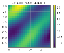
pred_labels = observed_pred.mean.view(n, n)
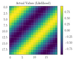
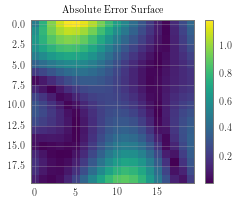
# Calc abosolute error
test_y_actual = torch.sin(((test_x[:, 0] + test_x[:, 1]) * (2 * math.pi))).view(n, n)
delta_y = torch.abs(pred_labels - test_y_actual).detach().numpy()
# Define a plotting function
def ax_plot(f, ax, y_labels, title):
if smoke_test: return # this is for running the notebook in our testing framework
im = ax.imshow(y_labels)
ax.set_title(title)
f.colorbar(im)
# Plot our predictive means
f, observed_ax = plt.subplots(1, 1, figsize=(4, 3))
ax_plot(f, observed_ax, pred_labels, 'Predicted Values (Likelihood)')
# Plot the true values
f, observed_ax2 = plt.subplots(1, 1, figsize=(4, 3))
ax_plot(f, observed_ax2, test_y_actual, 'Actual Values (Likelihood)')
# Plot the absolute errors
f, observed_ax3 = plt.subplots(1, 1, figsize=(4, 3))
ax_plot(f, observed_ax3, delta_y, 'Absolute Error Surface')
[ ]: